

Position Sizing in Directional Macro: A Practitioner’s Primer
Foundations: Volatility, Correlations, Regime Uncertainty, and Portfolio Survival


Executive Summary
Risk is the speed limit in directional macro. Forecasts about growth vs inflation, policy, flows, and catalysts are necessary to generate edge, but they are not what determines survival. Expected returns tend to evolve slowly through persistent “states” (macro regime, risk premia, momentum), while the risk environment (volatility and cross-asset dependence) can reprice abruptly. One can be driving in the right direction but still lose control by speeding into a sharp bend.
Volatility targeting is the discipline that keeps the book alive. Scaling positions inversely with estimated risk and targeting a portfolio-level volatility prevents risk from exploding in turbulent moments. Static frameworks like the 60/40 portfolios can unintentionally do exactly that: adding exposure into drawdowns when vol is highest.
After-shocks and correlation tightening punish over-reactive models. Post-shock relief rallies often tempt premature re-risking, but regimes are hard to observe in real time and stress frequently arrives in waves. In multi-asset portfolios, deleveraging and risk constraints can force simultaneous selling across positions, raising correlations and collapsing diversification. Because short-window correlation estimates are noisy, the robust approach is to adjust volatility more aggressively, estimate correlations with longer memory and shrinkage, and actively manage risk at the portfolio level.
Risk as the speed limit
Directional macro is often described as forecasting or predicting growth vs inflation, policy reaction functions, balance-of-payments, political catalysts. Of course, there’s no directional trading without predictions. But the quality of the predictions (or the hit rate) does not determine whether a macro book survives.
What matters most is risk management under regime uncertainty. Expected returns evolve slowly, while volatility and correlations can reprice in a day.
Durable macro performance is driven less by predicting returns (and certainly less by predicting regime shifts), and more by continuous portfolio resizing as the volatility environment changes. This concept is supported by a deep literature on volatility dynamics, long memory, regime switching, and time-varying correlation.
1. Expected returns drift; risk jumps
Merton (1980) argues that expected returns are extremely noisy to estimate and are not reliably identifiable from short-horizon data. Expected returns do change, but typically through slow-moving state variables—such as growth–inflation dynamics, policy regimes, momentum, or broader risk premia—and rarely through abrupt, discrete jumps.
Volatility is also known to exhibit persistence and long memory. A large literature documents that shocks to volatility decay slowly, with conditional variance displaying strong serial dependence over extended horizons (Ding–Granger–Engle (1993); Baillie–Bollerslev–Mikkelsen (1996)).
But at the same time, volatility also contains a fast-moving component. New information can reprice risk abruptly, producing large discrete jumps in realized and implied volatility. Corsi’s HAR framework (2009) provides a useful representation of this structure by decomposing realized volatility into daily, weekly, and monthly components.
So, while expected returns are difficult to estimate precisely over the near term, volatility can be measured and forecast with far greater statistical precision, as it exhibits pronounced clustering and serial dependence (Andersen et al., 2006).
A practical expression of this insight is found in industry risk models. In the RiskMetrics EWMA framework (Mina & Xiao (2001); MSCI RiskMetrics (2006)), a common daily decay factor of λ = 0.94 implies a volatility-shock half-life measured in weeks rather than years. Risk is explicitly designed to adapt quickly, even though it remains persistent.
The sizing implication is straightforward: macro theses can remain valid while the risk regime changes violently. Expected returns drift; risk jumps. The risk state is the faster-moving object and deserves more frequent attention in portfolio construction.
As an example, the below chart shows my return signals and expected volatilities over the last 10 years for 3 selected assets: Gold, Nasdaq, and 10-year JPY rates.
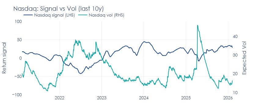
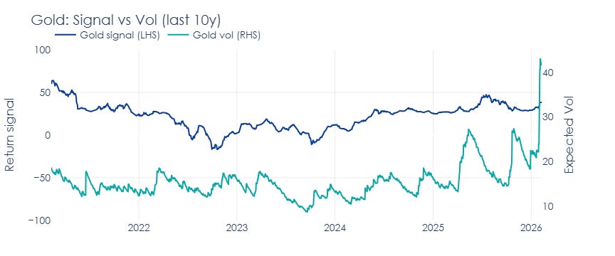
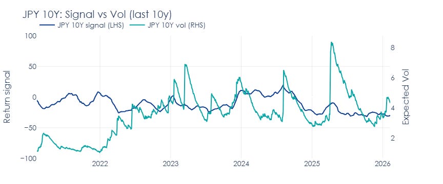
Now, let’s turn to the remaining aspects that matter for ongoing position adjustments and portfolio management: volatility targeting, regime shifts, vol-of-vol, and shifting correlations.
2. Volatility targeting is not optional
Volatility targeting is the first-order correction: scale positions inversely with estimated risk, and target volatility at the portfolio level. The goal is to prevent the portfolio’s risk from mechanically exploding when uncertainty rises.
Moreira & Muir (2017) show that volatility scaling (taking less exposure when volatility is high) can improve risk-adjusted performance across a range of asset classes and strategies. High volatility regimes carry higher crash risk, so holding constant exposure can become an impediment to compounding.
Not adjusting sizing when volatility rises is a deliberate decision to take more risk at a dangerous time - akin to speeding into a sharp bend.
Case study: The practice of asset allocation
Traditional balanced portfolios (e.g., 60/40) are typically implemented with calendar or threshold rebalancing and implicit long-run assumptions about volatilities/correlations being “reasonable” most of the time.
But when those assumptions break, the rebalancing process can become an accidental pro-risk rule: it adds exposure into drawdowns precisely when risk is elevated.
The mismatch gets worse when “tactical” overlays are justified by valuation-based return forecasts. Goyal & Welch (2008) show that many popular equity-premium predictors perform poorly out of sample and appear unstable—casting doubt on the idea that expected returns reliably “jump” enough during drawdowns to justify taking more risk.
The chart below highlights the deep drawdowns in the US 60/40 equity/bond portfolios which could have been reduced if the 30-day trailing volatility was used actively as a “speedometer”, instead of allowing the gross exposure to remain static while volatility explodes.
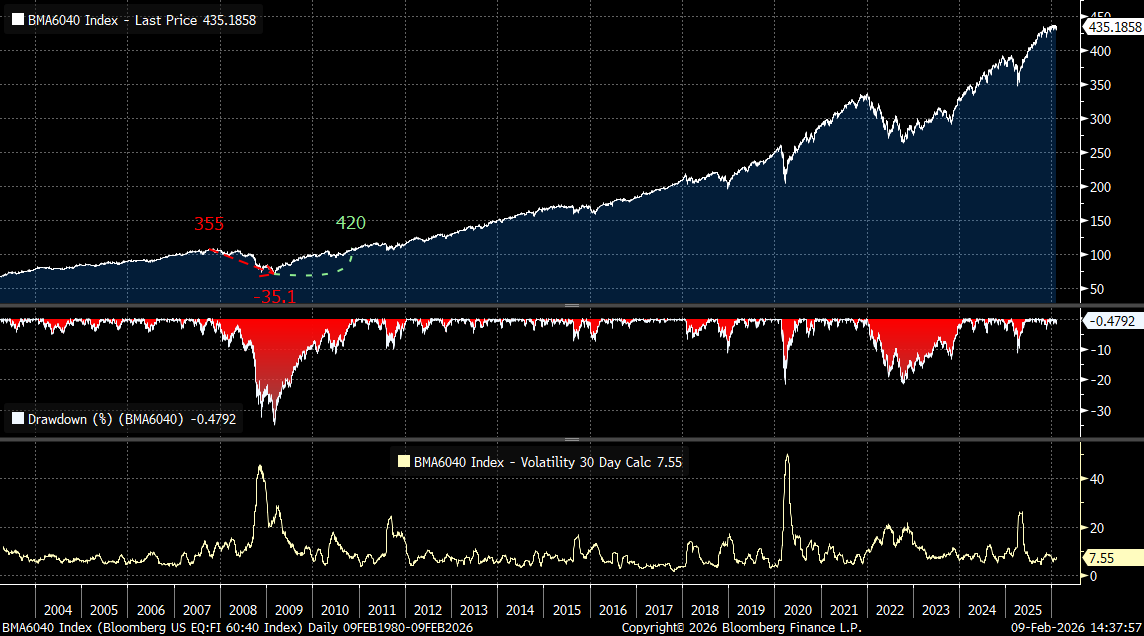
For completeness - this does not necessarily mean allocators are irrational. In many contexts, they face constraints around mandates, derivatives restrictions, governance, and size. But from a macro trader’s viewpoint, it is critical to see the mechanical mismatch: static exposure implicitly assumes risk is roughly stable, while markets are repeatedly telling us it isn’t.
The practical implication is that it is often ok to keep a thesis on in times of stress, but it is not ok to keep the sizing that belongs to a different regime.
3. The second-order problem: vol-of-vol and regime mixtures
After the first volatility spike, markets often stage relief rallies: liquidity improves, prices retrace, realized volatility compresses for a few sessions. That often creates a temptation to re-risk quickly (or buy-the-dip). Then the second wave hits, correlations snap tighter, and the portfolio is oversized again.
Engle & Patton (2001) frame volatility as a conditional process with features that a usable model should capture, including persistence, mean reversion and asymmetry. The practical takeaway is the one that traders learn the hard way: post-shock volatility does not normalize smoothly or symmetrically.
Returns are often better described as coming from a mixture of distributions rather than a single stable process. Hamilton’s (1989) regime-switching framework formalizes time series as switching between latent states with different statistical properties. Ang & Timmermann’s (2012) review makes the broader point: financial markets can change behaviour abruptly and the new behaviour can persist. Ignoring regimes can lead to systematic mismeasurement of risk.
This is where the trader’s lived experience (“relief rally → renewed stress”) meets the statistician’s representation: state dependence plus unobservability of the state in real time. If I cannot reliably observe the regime, the sizing rule must be robust to being wrong.
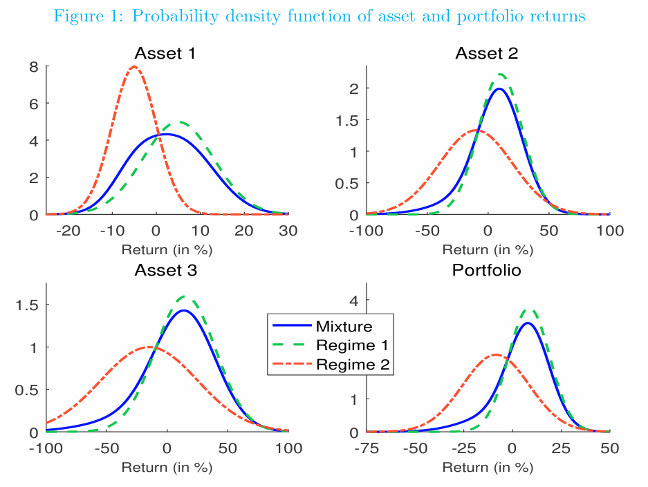
The figure below from Lezmi et al. (2019) provides a particularly usable framing for practitioners: model returns as a two-regime Gaussian mixture—a “normal” regime (green) and a “turbulent” regime (red) —then treat skewness/crash risk as arising from the stress component’s weight and parameters.
4. After-shocks and unpredictability of regime switching
A common reaction to regime ambiguity is to make the risk model “faster”: shorter lookbacks, higher responsiveness, more aggressive filters. Intuitively it feels safer. In practice it can become procyclical:
volatility compresses briefly → model declares “normal” → sizing increases
stress resumes → correlations rise / volatility returns → drawdown accelerates
This is a modelling error: confusing a short lull inside a stress episode for a genuine regime change. The long-memory evidence (HAR-type models; FIGARCH-type representations) tells us that volatility shocks can decay more slowly than a short-horizon filter assumes.
From a market-microstructure perspective, large positions are rarely unwound in a single move. Inventory reduction tends to occur in phases, as liquidity allows and prices recover sufficiently to facilitate further selling. What technicians often describe as a “distribution phase” is simply the visible manifestation of this process: risk being transferred gradually, not instantaneously.
Seen through this lens, short-term volatility compression during stress should not be interpreted as confirmation that the regime has normalized. It is often just a pause in the unwinding process. Risk models that respond too quickly to these pauses end up increasing exposure precisely when the probability of renewed stress remains elevated.
In real time, we cannot know how much inventory is left to be unloaded during the stress phases and how many more forced sellers are holding their positions. Even the most successful technical analysts leave a lot of room for error in their predictions around move extensions via sizing. In quant literature, betting on regime switches is simply too dangerous, and sizing for a possibility of after-shocks via a well-calibrated volatility estimate is the most practical and widely used strategy.
5. Correlation estimates are too noisy
In principle, multivariate GARCH models give an elegant answer to time-varying cross-asset risk: volatility and correlations can both move through time. Engle’s Dynamic Conditional Correlation model (DCC) is the canonical framework (Engle (2002)), building on the broader conditional-variance tradition (Bollerslev (1986)).
The microstructure intuition reinforces the point. During deleveraging episodes, margin constraints and risk limits force players to cut multiple positions at once—including “non-problematic” ones—which mechanically increases co-movement and drives correlation spikes (Kyle & Xiong (2001); Brunnermeier & Pedersen (2009)).
In practice, however, estimating a fast-moving covariance matrix is often the weak link. The core issue is statistical: with N assets there are (N^2-N)/2 off-diagonal covariance (correlation) terms, and those cross-terms are typically far noisier than the diagonal volatility estimates at the horizons traders care about.
As a result, sample covariance matrices can be unstable or ill-conditioned, and attempts to update correlations too actively add more noise and turnover than genuine information.
This is why shrinkage and regularization are widely recommended for stability and out-of-sample performance (Ledoit & Wolf (2003, 2004)), and why the empirical correlation structure is often described as containing a substantial noise component at typical sample sizes (Laloux et al. (1999); Plerou et al. (2002)).
That does not mean correlations don’t matter. In stress, diversification deteriorates because dependence tightens. But rather than trying to infer this from noisy short-window correlation estimates, it is often more robust to:
update vol more aggressively (diagonal terms are easier to estimate),
update correlations more conservatively with longer memory and shrinkage, and
manage risk at the portfolio level when conditions become unstable.
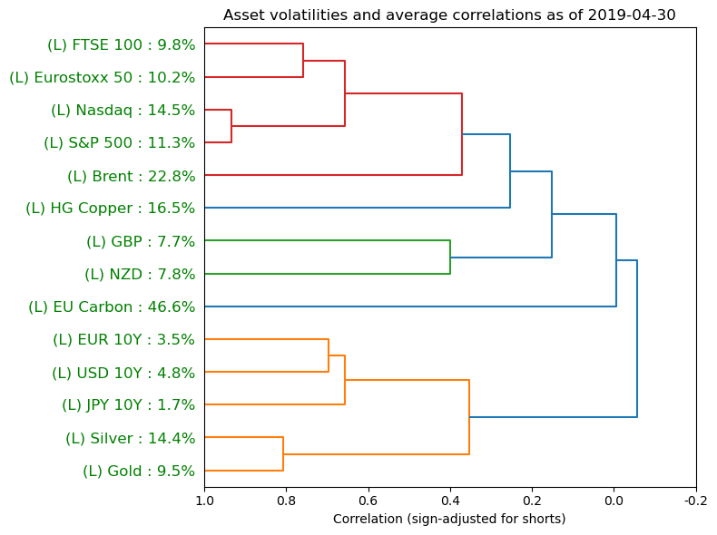
The dendrograms I show below come from my multi-asset risk model and reveal that my correlation estimates do not change as much as volatilities as regimes shift between calm (top chart) and stressed (bottom chart).
6. My implementation principles
The literature converges on principles that match trading reality.
Update risk estimates on a daily basis.
Not because we can predict daily vol with high accuracy (we cannot), but because the alternative is letting a nonstationary system drift away from the book’s risk budget. Volatility is measurable and persistent. Ignoring it is the sure route to overexposure.De-risk faster than I re-risk.
The logic comes from vol-of-vol and regime mixtures: after a shock, uncertainty about the regime is elevated, and after-shocks are a possibility. As a result, I treat early “calm days” as weak evidence.Tolerate ambiguity instead of trying to time the switch.
Models can describe regime behaviour, but they do not give me a live trading oracle. The market can ping-pong between regimes on horizons too short for clean classification, so my sizing rule must survive being too early or too late.Equity-curve smoothness enables compounding.
Deep drawdowns are a huge operational problem. Volatility scaling is ultimately about staying solvent and functional through repeated stress cycles—so that I’m able to raise my stakes again when the opportunity set improves.
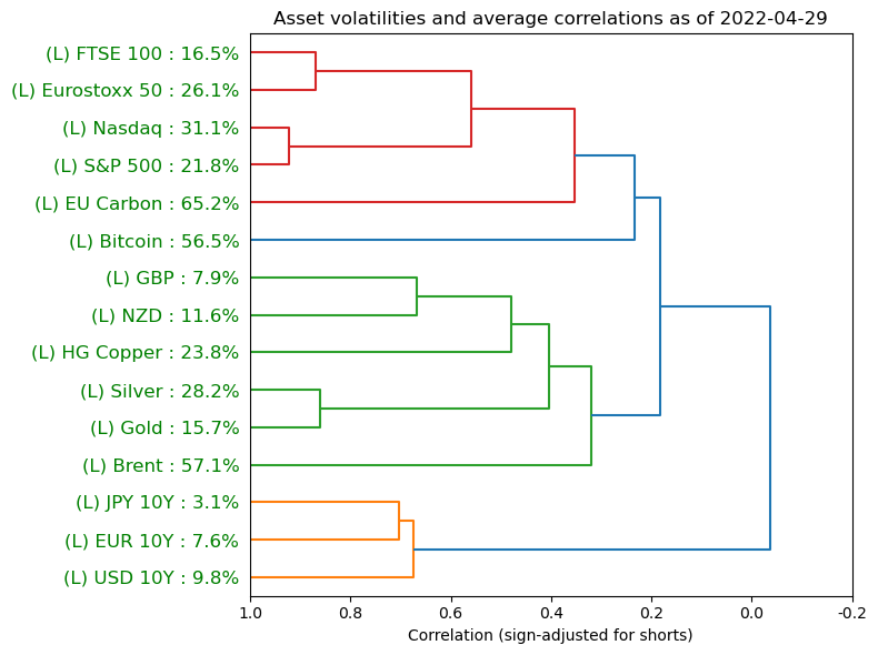
As a final illustration, below is the scatter of expected multi-asset volatility and actual total gross exposures for the vol-adjusted portfolio that I cover in my Quant Playbook. The slope of the scatter implies smaller positions in times of high volatility. The methodology underneath this systematic portfolio incorporates all concepts from this article, including vol scaling of positions, vol targeting at portfolio level, acknowledging the risk of after-shocks, and correlation adjustment.
Conclusion: survival above all
In directional macro, it’s tempting to believe that the edge is being right about the next catalyst. Sometimes it is. But over a career span, this edge is not sufficient.
Keeping the risk budget relatively stable across repeated volatility cycles is a necessary condition for survival. That is what keeps me at the table to play the next hand. That requires accepting a simple, non-glamorous truth: I cannot control the regime, I cannot observe it perfectly in real time, and I cannot force volatility to behave politely. What I can control is sizing.
When volatility rises, I resize the whole portfolio to survive. When volatility feels lower soon after the shock, I assume that’s the dangerous moment—not automatically the all-clear. No speeding into sharp bends.
References
Merton (1980) — On Estimating the Expected Return on the Market: An Exploratory Investigation. Journal of Financial Economics, 8(4), 323–361.
Andersen–Bollerslev–Diebold–Christoffersen (2006) — Volatility and Correlation Forecasting. In Handbook of Economic Forecasting, Vol. 1 (Elsevier), Chapter 15, pp. 777–878.
Mina & Xiao (2001) — Return to RiskMetrics: The Evolution of a Standard. RiskMetrics Group.
MSCI RiskMetrics (2006) — The RiskMetrics 2006 Methodology. MSCI / RiskMetrics (technical documentation).
Corsi (2009) — A Simple Approximate Long-Memory Model of Realized Volatility. Journal of Financial Econometrics, 7(2), 174–196.
Ding–Granger–Engle (1993) — A Long Memory Property of Stock Market Returns and a New Model. Journal of Empirical Finance, 1(1), 83–106.
Baillie–Bollerslev–Mikkelsen (1996) — Fractionally Integrated Generalized Autoregressive Conditional Heteroskedasticity. Journal of Econometrics, 74(1), 3–30.
Moreira & Muir (2017) — Volatility-Managed Portfolios. The Journal of Finance, 72(4), 1611–1644.
Engle & Patton (2001) — What Good Is a Volatility Model? Quantitative Finance, 1(2), 237–245.
Hamilton (1989) — A New Approach to the Economic Analysis of Nonstationary Time Series and the Business Cycle. Econometrica, 57(2), 357–384.
Ang & Timmermann (2012) — Regime Changes and Financial Markets. Annual Review of Financial Economics, 4(1), 313–337.
Lezmi et al. (2019) — Portfolio Allocation with Skewness Risk: A Practical Guide. SSRN working paper / preprint (Lyxor/Amundi quant research line).
Bollerslev (1986) — Generalized Autoregressive Conditional Heteroskedasticity. Journal of Econometrics, 31(3), 307–327.
Engle (2002) — Dynamic Conditional Correlation: A Simple Class of Multivariate GARCH Models. Journal of Business & Economic Statistics, 20(3), 339–350.
Goyal & Welch (2008) — A Comprehensive Look at the Empirical Performance of Equity Premium Prediction. The Review of Financial Studies, 21(4), 1455–1508.
Campbell & Shiller (1988) — The Dividend-Price Ratio and Expectations of Future Dividends and Discount Factors. The Review of Financial Studies, 1(3), 195–228.
Cochrane (2008) — The Dog That Did Not Bark: A Defense of Return Predictability. The Review of Financial Studies, 21(4).
Kyle & Xiong (2001) — Contagion as a Wealth Effect. The Journal of Finance, 56(4), 1401–1440.
Brunnermeier & Pedersen (2009) — Market Liquidity and Funding Liquidity. The Review of Financial Studies, 22(6), 2201–2238.
Ledoit & Wolf (2003) — Improved estimation of the covariance matrix of stock returns with an application to portfolio selection. Journal of Empirical Finance, 10(5), 603–621.
Ledoit & Wolf (2004) — Honey, I Shrunk the Sample Covariance Matrix. The Journal of Portfolio Management, 30(4), 110–119.
Laloux–Cizeau–Bouchaud–Potters (1999) — Noise Dressing of Financial Correlation Matrices. Physical Review Letters, 83(7), 1467–1470.
Plerou et al. (2002) — Random Matrix Approach to Cross Correlations in Financial Data. Physical Review E, 65, 066126.
Disclaimer
Convexta does not provide dealing, solicitation, or advisory services in futures or securities, and does not offer asset management services. All publications are made available to the public. Authors’ personal allocations and opinions are provided for educational purposes only, are not tailored to any specific reader, and do not constitute investment advice.